Sine and Cosine

Over the years, I have seen many students struggle with Sine and Cosine. It is easy to understand why: These words seem rather scary and abstract, especially if you do not consider yourself good at math. However, this is both unfortunate and unnecessary. Unfortunate, because these two functions are a fundamental part of most programmatic designs, and a good understanding of them will allow you to solve many visual problems. Unnecessary, because they are not that hard to learn. Even if you do not understand everything presented in this chapter, you can get started by memorizing two almost identical lines of code.

Sine and Cosine allow us to find any position on the outline of an ellipse. They do this by converting an angle into an x position (Cosine) or a y position (Sine) for a circle with a 1 pixel radius. These values can then be multiplied by the radius of your actual circle to scale them up. Although it is not strictly necessary to understand how these functions work internally, here is a way to visualize what is going on: Imagine a right sided triangle connecting the center of the circle to the point on the outline. The Sine function is a quick way to get the ratio between the left side (hypotenuse) and the right side (opposite) of that triangle. The Cosine function is likewise the ratio between the hypotenuse and the bottom side (adjacent) of the triangle.

In P5, these functions are called sin() and cos(). As described above, they accept a single argument – an angle in radians – and return a value between -1 and 1 representing the x or y position on a tiny circle. The two lines below demonstrate how to get these values and multiply them by the radius of your actual circle. Memorize these two lines, as they are very important.

const x = cos(RADIANS) * RADIUS;
const y = sin(RADIANS) * RADIUS;

To put this into context, here is an example where we use the same code to draw a small circle 330 degrees along the outline of a bigger circle.

translate(width/2, height/2);

noFill();
const radius = width * 0.3;
ellipse(0, 0, radius*2, radius*2);

fill(30);
const x = cos(radians(330)) * radius;
const y = sin(radians(330)) * radius;
ellipse(x, y, 20, 20);

If you consider all the basic shapes – as well as many complex shapes – they are characterized by having non-overlapping outlines that move around a center point. Some shapes, like the triangle, have just a few vertices, while others – like the ellipse – have many vertices. The sin() and cos() functions give a way to procedurally draw these types of shapes.

The For Loop

Although we will dedicate an entire part of this book to repetition, let us briefly go over the basic functionality of a for loop. A for loop allows us to execute code multiple times in a row by incrementing (or decrementing) a variable – often called i – until an expression is no longer true and the loop stops. In the following example, we initialize a variable with the number 0, iterate as long as our variable is lower than 10, and increment our variable by one between each iteration. The result is a loop that iterates ten times with our variable incrementing from zero to nine, drawing ten rectangles on the screen.

for(let i = 0; i < 10; i++) {
  rect(0, 0, 100, 100);
}

Unfortunately, all these rectangles have identical positions and sizes because we are passing the same static numbers to the rect() function over and over again. This is where i comes into play: Because it changes between each iteration of the loop, it can be used to create variance between each rectangle. The example below uses i to position the ten rectangles one pixel apart on the x-axis.

for(let i = 0; i < 10; i++) {
  rect(i, 0, 100, 100);
}

Although it might not be immediately clear, this is an important technique when drawing procedural designs. Because i increments by one between each iteration, it can be used as a scalar to distribute shapes across the canvas. For example, if we want to position the rectangles next to each other, we can multiply i with a number greater than the width of the rectangles.

for(let i = 0; i < 10; i++) {
  rect(i * 105, 0, 100, 100);
}

We can use this same technique to draw custom shapes. Instead of drawing individual shapes in the loop, we use the for loop to procedurally add vertices between the beginShape() and endShape() function calls. In the example below, we use this technique to draw ten random vertices in the center of the canvas.

translate(width/2, height/2);
beginShape();
for(let i = 0; i < 10; i++) {
  const x = random(-100, 100);
  const y = random(-100, 100);
  vertex(x, y);
}
endShape();

The result is certainly a procedural shape, but the use of random() does not give us a lot of control over the placement of the vertices: The shape is just a bunch of lines randomly crossing each other. The final step is to put our two techniques together and generate shapes with sin() and cos() inside of a for loop.

Putting it together

Starting from our random shape code above, let us replace the random vertices with vertices placed sequentially along the outline of an ellipse. We do this by using the same two lines that we memorized earlier, but instead of passing the same angle to sin() and cos(), we calculate a different angle on every iteration by multiplying i with the angle we want between the vertices. The result is a shape with ten vertices evenly spread around the center of the canvas.

translate(width/2, height/2);
beginShape();
for(let i = 0; i < 10; i++) {
  const x = cos(radians(i * 36)) * 100;
  const y = sin(radians(i * 36)) * 100;
  vertex(x, y);
}
endShape();

By changing the number of iterations and the spacing between the vertices, you can draw all of the basic shapes. The code below adds a few variables on top of the sketch to automatically calculate the spacing based on the number of vertices. Change the numVertices variable and another shape will appear.

const numVertices = 3; // or 4 or 30
const spacing = 360 / numVertices;
translate(width/2, height/2);
beginShape();
for(let i = 0; i <= numVertices; i++) {
  const x = cos(radians(i * spacing)) * 100;
  const y = sin(radians(i * spacing)) * 100;
  vertex(x, y);
}
endShape();

‘Great, we have reinvented the basic shape functions’ you might say. Actually, this technique allows us to draw much more sophisticated shapes. Let's run through a few examples that all use the same sin() and cos() formula to draw different types of shapes. We'll start with the squiggly circle below that has a random radius for each vertex, making it look like it was drawn by hand.

translate(width/2, height/2);

beginShape();
for(let i = 0; i < 100; i++) {

  const radius = 100 + random(5);

  const x = cos(radians(i * 3.6)) * radius;
  const y = sin(radians(i * 3.6)) * radius;
  vertex(x, y);
}
endShape();

The star below is created by alternating between a low and a high radius for each vertex. It's easy to tweak the style of the star by using different numbers or more vertices, or using rotate() to change the orientation of the star.

translate(width/2, height/2);

let radius = 100;

beginShape();
for(let i = 0; i < 10; i++) {

  const x = cos(radians(i * 36)) * radius;
  const y = sin(radians(i * 36)) * radius;

  vertex(x, y);

  if(radius == 100) {
    radius = 50;
  } else {
    radius = 100;
  }

}
endShape();

Here is a flower created with quadraticVertex() where all vertices and control points are positioned using sin() and cos(). By using a larger radius for the control points (the inverse of the star example above), the curves go outwards. When using Bézier curves, remember to start the shape with a vertex() function call. We do this by checking the value of i within the loop.

translate(width/2, height/2);

const numVertices = 7;
const spacing = 360 / numVertices;

beginShape();

for(let i = 0; i < numVertices+1; i++) {

  const angle = i * spacing;
  const x = cos(radians(angle)) * 100;
  const y = sin(radians(angle)) * 100;

  if(i == 0) {

    vertex(x, y);

  }
  else {

    const cAngle = angle - spacing/2;
    const cX = cos(radians(cAngle)) * 180;
    const cY = sin(radians(cAngle)) * 180;
    quadraticVertex(cX, cY, x, y)

  }
}
endShape();

You will often find yourself needing to use just one of the circular functions. The two shapes below are created just like that: The first one uses sin() and the second one uses cos() (as demonstrated in the code below).

strokeWeight(20);
strokeCap(SQUARE);
translate((width/2) - 200, height/2);
beginShape();
for(let i = 0; i < 200; i++) {

  const x = i * 2;

  const y = cos(i * radians(2)) * 100;

  vertex(x, y);
}
endShape();

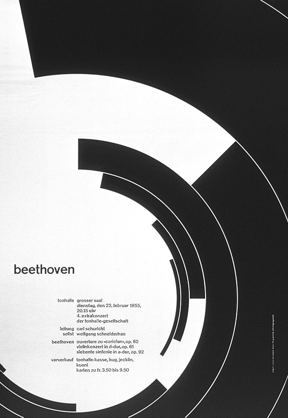
Sine and Cosine can be used to create a range of different shapes during the design process. In this design by Josef Müller-Brockmann, a series of exponentially growing arcs are rotated around the bottom left of the canvas.

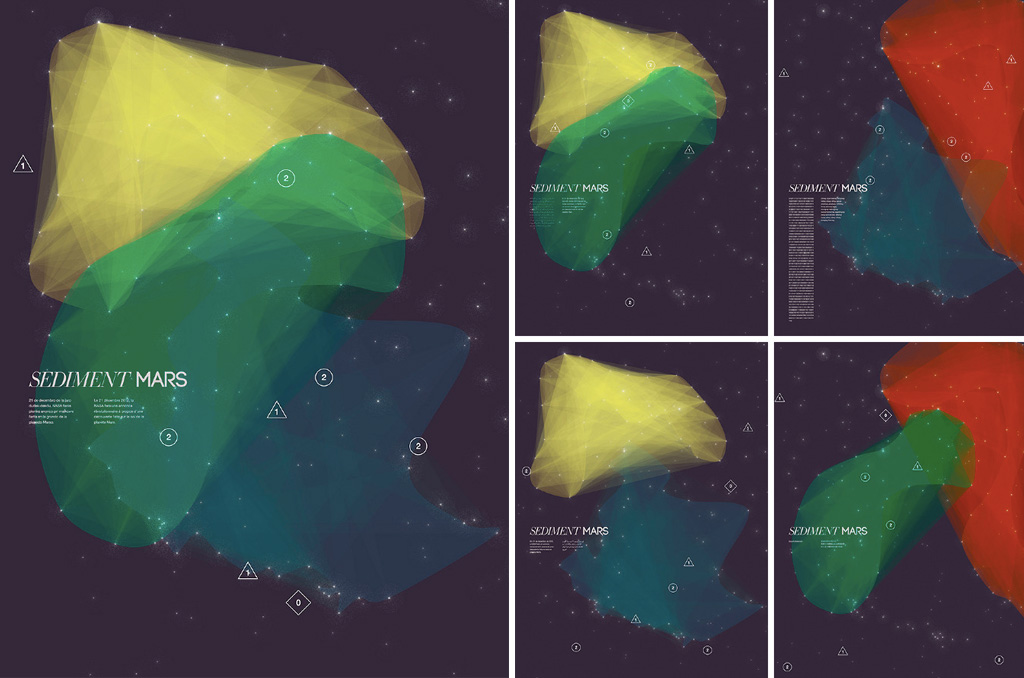
Sediment Mars is a series of generative poster designs by Sarah Hallacher and Alessandra Villaamil. The sin() and cos() functions are used to generate an elliptical shape, which is then distorted by adding random values to it.

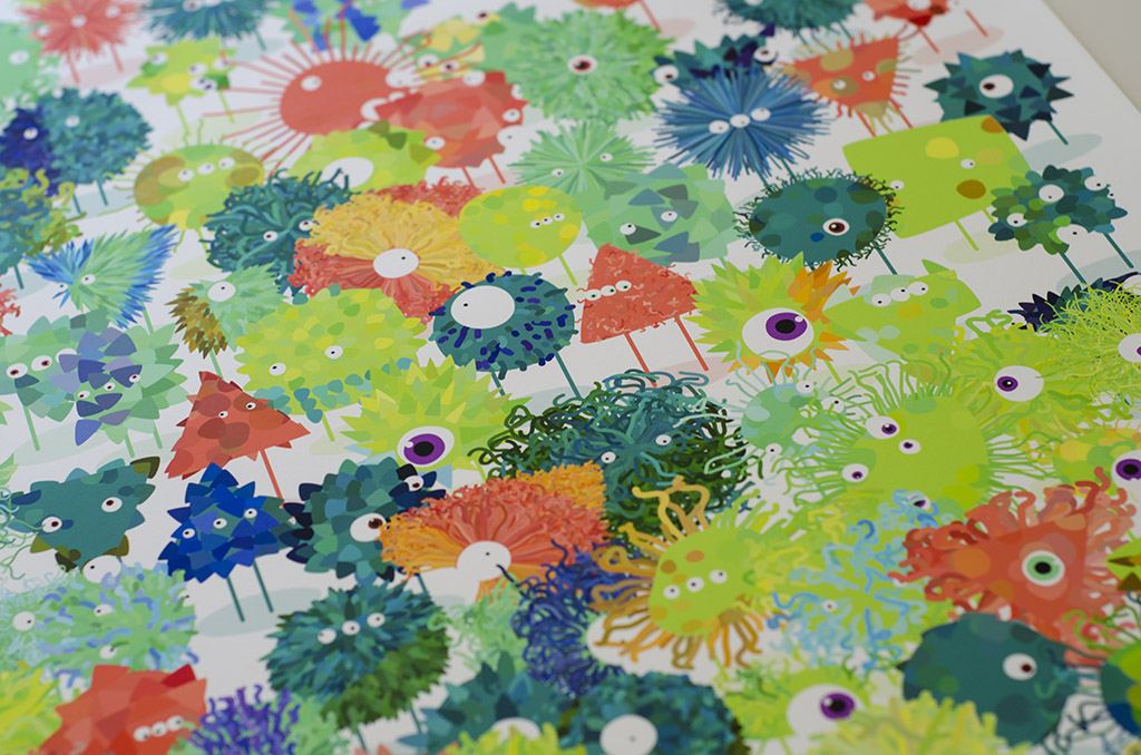
The project Generative Play is a card game by Adria Navarro that uses procedural drawing to create an infinite amount of generative characters. The character bodies are created using sin() and cos().

This chapter introduced an approach to design that is inherently different than a traditional design process. Rather than individually placing each shape on the canvas, we wrote algorithms to do this for us. Using loops to procedurally draw shapes is a powerful concept, as it allows designers to do more with less code, thus alleviating us from the pains of manually constructing every design object by hand. This is also the hardest thing about procedural design, as designers need to devote more time up front distilling the system into code, and they cannot easily manipulate individual shapes like in a traditional design tool. The American computer scientist Donald Knuth calls this a transition from design to meta-design:

“Meta-design is much more difficult than design; it is easier to draw something than to explain how to draw it. […] However, once we have successfully explained how to draw something in a sufficiently general manner, the same explanation will work for related shapes, in different circumstances; so the time spent in formulating a precise explanation turns out to be worth it.”

Donald Knuth (1986), The Metafont Book

This is also the main thesis of this book. When designers learn to not only think systematically about the design process, but also to implement those systems in software, they can build things that were not possible before.